Transit Planner
An experiment on transfer patterns robustness in the presence of real-time updates
Implementation of the Transit Planner
This chapter provides detailed information on the components of our implementation of transfer pattern routing for transit networks. We present the algorithms and data structures used to compute and store transfer patterns and to answer shortest-path queries. Finally we explain how we model real-time updates based on a modification of GTFS-metadata.
Transit Network Construction
We use a custom GTFS-parser to translate a transit feed into a graph, which is used to compute transfer patterns and run reference shortest-path searches. In a first step, we collect information on stops and the set of trips with activity information, time-labeled stop sequences and a frequency. We keep this metadata, for the modeling of the dynamic trip delays during the experiments.
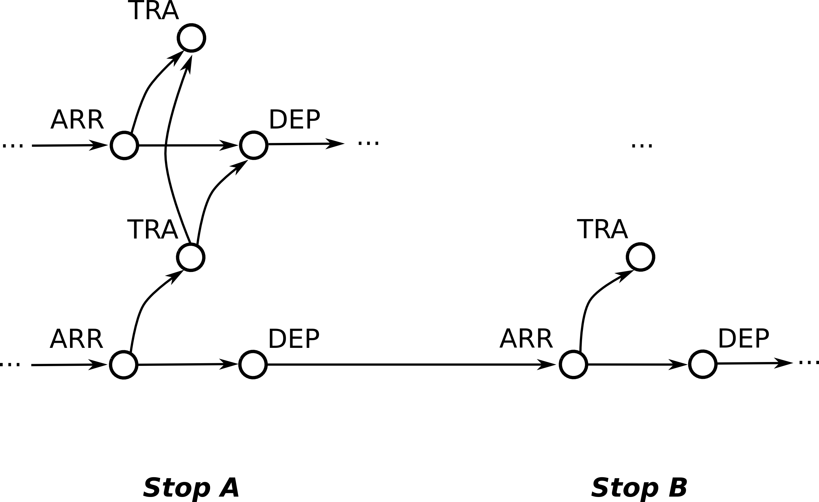
The second step translates the metadata into a time-expanded transit network of nodes and connecting arcs. Every node comes with a timestamp and each arc has a multi-criteria cost function: the time of travel in seconds and an integer penalty to denote transfers. For each incidence of a trip at a stop, the transit network contains three nodes: one arrival node, one departure node and one transfer node. There is an arc between the arrival and the departure node and one from the arrival to the transfer node. The former corresponds to the event of remaining in the vehicle, whereas the latter to exiting. Its cost is a time value equal for all transfers, called transfer buffer, and it has a penalty of one.
Along a trip, successive stops are connected by an arc between the departure and arrival node. The cost of each arc is determined by the timestamp difference of the adjacent nodes. To model transfer from one vehicle to another, among the nodes of every stop each transfer node is connected to all succeeding departure nodes up until the next transfer node, to which there is an arc as well.
Due to the nature of public transportation organisation, GTFS-feeds for the same location are provided by multiple agencies. Therefore, Transit Planner's GTFS-parser can parse multiple feeds and combine them effectively into one transit network.
Through proper modularization of the parser, we are able to reuse it for the generation of the experimental delay scenarios. More details on this is provided in the description of the scenario generator.
Walking Graph
Our network representation has a drawback for practicability: imagine you get off a bus and walk over the street to take the tram going in the opposite direction. Our network so far has no means of modeling this.
To overcome this, we maintain an additional walking graph. The walking graph connects each stop to stops nearby with an arc of costs corresponding to the approximate walking time. For every stop we add such a walking arc to every other stop within a constant distance. We keep the walking graph separate in order not to blow up the transit network. In shortest path searches the walking graph is used differently depending on whether a Dijkstra or transfer pattern query is performed. Further information on the usage of the walking graph is provided in the corresponding sections.
To avoid paths consisting mainly of walking arcs, we forbid subsequent walking. In transit networks with a high concentration of stops in small areas this expansion step would massively enlarge the search space and thus the number of transfer patterns. The maximal distance of 100 meters for allowed walkways has been chosen according to hardware restrictions for the precomputation.
Shortest-Path Search
To find shortest paths in the transit network, respectively optimal connections between two stops at a certain time, we use Dijkstra’s algorithm. It is used for computing the transfer patterns in the precomputation as well as reference shortest path to compare to the transfer pattern search in the experiments on modified networks.
Our implementation uses a multi criteria cost function maintaining time and penalty on labels which are associated to nodes in the transit network. Each node may have several labels with different penalty values which belong to different paths traversing that node. Detailed information on how the labels are maintained is given in a later section.
The expansion of labels distinguishes two cases: The expansion of arcs in the transit network and the expansion of arcs in the walking graph. The former creates labels at successors nodes reached by the outgoing arcs of the current node in the transit network. The latter gets all stops connected in the walking graph with the stop of the current node. For each of these stops the matching start node sequence in the transit network is identified, comprising all departure nodes until the first transfer node with time stamps higher than the previous label’s costs plus walking cost and transfer buffer. For all these nodes new labels are pushed in the priority queue.
The Dijkstra is used to find shortest paths between a pair of departure and destination stops as reference in the experiment evaluation (see section on experiments) and to compute the transfer patterns in the precomputation. For the latter use case a termination criterion is enabled, which stops the search when all open paths run over a hub stop.
Precomputation
In the first step of the precomputation we use a time-compressed variation of the transit network to select the 1% most important stops as hubs. We investigated various selection strategies. However, as stated in the literature [citation Bast et al.], the choice of hubs has only marginal influence on the performance so we stick to the simplest method: We run a number of full Dijkstras from random stops counting the number of optimal paths transferring at each stop and select the stops with the highest number of transfers.
For every hub we run a complete Dijkstra on the transit network. For the other stops the Dijkstra search ends when all of its open paths have run over a hub stop. To avoid suboptimal paths and to reduce the size of the transfer pattern database we run the arrival loop algorithm for each stop. Such paths evolve from the fact that in transit networks, other than in road networks, each arc is on a shortest path. In principle that algorithm scans for each stop if there are labels at arrival nodes which could be reached by waiting from previously reached labels and removes the former.
We backtrack paths from all destination stops, starting from labels at arrival nodes as well as walking labels at transfer and departure nodes. Along each path we collect the stops where transfers occur. For each pair of departure and destination stops we store these sequences as transfer pattern.
LabelMatrix
The shortest path search is based on the multi-criteria labels and is critical for the efficiency of the transfer patterns precomputation. Since the priority queue operations are the bottleneck of the Dijkstra algorithm, an efficient data structure for the multi-criteria labels is mission-critical.
A label holds the tentative cost and penalty value of a node. Due to the Pareto-optimality, multiple mutually incomparable labels can be simultaneously assigned to a node. The most important requirement of the label container is an efficient optimality test given an new candidate label with respect to all the labels already contained.
Our first approach to label maintenance was the space-efficient LabelSet. Its tree-based structure held the labels sorted by cost and provided optimality test in logarithmic time. However due to the high throughput and the inherently cache-inefficient label distribution, this data structure did not perform sufficiently well on big datasets.
Under the consideration that the penalty upper bound is always a small number (less than 10), it was viable to expand the memory allocations to hold all possible penalty values for a given cost. This allowed us to implement the LabelMatrix, which is a vector of fully penalty-expanded label vectors. The LabelMatrix is less space-efficient compared to the LabelSet, but it provides all critical operations in constant time relative to the maximum penalty value.
Transfer Patterns Graph
During the transfer patterns precomputation we collect optimal sets of transfer patterns for every source station and store them in a compressed directed acyclic graph called transfer patterns graph, TPG for short. For each transfer pattern from a given departure to a destination stop there is one reversed path in the TPG of the departure stop.
The TPG data structure is path-prefix aware, meaning it interleaves common path prefixes to reduce the total space consumption. This data structure is based on the proposal in [1].
Query Graph
At query time, transfer pattern based routing does not depend on the original transit network. To answer queries between a departure stop and a destination stop a temporary query graph is created. It can be regarded as a concise representation of the network of direct connections between departure and destination stop.
It is constructed from the transfer pattern graph by backtracking paths from the destination node corresponding to the destination stop down to the root node. A stop contained in several different patterns, respectively contained several times in the TPG, is represented by just one node in the query graph. Arcs between the different stops represent time-dependent connections of the transfer pattern and are not labeled with costs.
Due to the use of hub stops in the precomputation, the destination stop is often not part of the elementary TPG of the departure stop. Therefore the query graph is constructed from the departure stop's TPG to every reachable hub and then extended with query graphs from each of the hubs to the destination stop.
It is worth noting that due to the one-to-one correspondence of the query graph's nodes to real stops a query graph constructed for a set of transfer pattern may comprise routes of suboptimal pattern. As an example, consider the query graph build for the pattern (A,B,C,D) and (A,C,B,D). In addition to the paths corresponding to these patterns, the graph contains the paths (A-B-D) and (A-C-D) which might be suboptimal. This matter becomes more important with the use of hubs. Consider the query graphs build for pattern (A-B-C-D-Hub) and (Hub-D-E-F-G) respectively. Both correspond to shortest paths with three transfers. But if you merge the graphs as described above, the resulting graph contains the path (A-B-C-D-E-F-G) which has five transfers without a hub. We implemented another approach where the distinct query graphs are linked rather than merged. Our experiments showed that this increases the time of pattern-based shortest path queries by a factor of two, while possibly suboptimal pattern as in the first example remain. So we sticked with the first approach.
Direct Connections
To process queries on the query graph efficiently, we need fast access to direct-connection costs between stops. A direct-connection is a transfer-free connection between two stops. The DirectConnection data structure is designed to answer such queries fast.
For that it is filled with all trips during the network construction. Trips serving the same sequence of stops without transfers are recognized as the same line. For each line a table is constructed with the respective trip times and stored in the DirectConnection data structure. Additionally, for each stop we store a lookup-entry called incidence list, with all the lines that serve the stop and the position of the stop in the lines’ sequences.
The lookup-table allows an efficient method to answer direct-connections queries: By intersecting the incidence lists of the given departure and destination stops, we retrieve all lines serving both stops of interest. In the next step, we filter out all lines, where the destination stop is served before the departure stop within the line’s sequence. The remaining incidence list contains all feasible connections and we choose the one with the minimal cost, i.e. the one arriving first at the destination. This data structure is based on the proposal in [1] where a detailed analysis can be found.
Short-Path Queries
After the query graph is constructed, a Dijkstra search can be used to find the shortest paths to the destination stop. Like the Dijkstra for transit networks the search on query graphs runs with a multi-criteria cost function (time and penalty) on labels, which are linked to stops in the query graph.
Instead of annotated time values at arcs the travel cost have to be computed online using the direct-connection data structure described above. The penalty value is increased by one with each expansion except for walking arcs, owing to the fact that each node traversed in the query graph marks a transfer in a shortest path between departure and destination.
Scenario Generator
In our experiments we want to examine the robustness of transfer patterns towards real-time updates. The most common use case of such updates are traffic delays. If there was delay in the network, we would like to know if the new optimal paths are still contained in the precomputed transfer patterns.
We model delay of connections on the base of single trips. Our generator delays a percentage of all trips in the following policy. For every trip to modify, we insert a constant delay after a uniformly chosen stop. The delay itself is sampled from an exponential distribution of user-specified mean. We define three types of delay: small (5 minutes), medium (15 minutes) and high (50 minutes mean). These values describe the arithmetic mean of the exponential distribution that generates the actual delay. So there are two parameters to modify the network: The percentage of trips to delay and the mean of the delay.
The figure illustrates the probability density functions for the three types of delay: small, medium and high: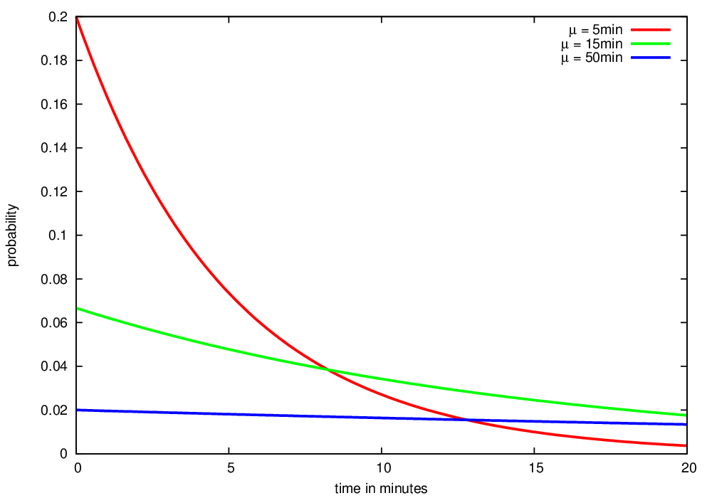
For our experiments we also use combined settings. For example we could delay 10% of all trips with 15 minutes and 5% with an average of 50 minutes delay.
Example output of the generator:
Inherent issues
During the implementation we made many decisions about the design of our software. Most of them were motivated by our focus on the experiments or to fullfill hardware and time constraints and most proved to be justified. However, after working on the project for many months we now know that some aspects about transit networks and routing with transfer patterns should be handled differently. We state some of our knowledge here along with a description of known but unsolvable (not within a reasonable amount of time) issues in order to make future programers and researchers aware of these problems.
The first issue is around the walking problem. Walking is natural for a person travelling in the real world. But from a programmers point of view, transit network routing with walking is much harder to implement in a reliable and consistent way. We decided to keep the walking graph separately from the transit network. This leads to a problem whenever multiple routes arrive at a destination stop by walking such that they enter at the same transfer/departure node: One of the paths will be lost. The unit-test TransferPatternRouterTest.walkTestCase4 gives a detailled example.
Nowadays we would not pursue the strategy of a separate walking graph any more. Rather than expanding walking arcs on the fly, we recommend to do this when constructing the transit network: For every arrival node expand walking arcs to neighboring stops and add a transit node with the correct time offset, connected by an regular arc. This way walking becomes the same thing as a transfer, which coincides with the intuitive notion: If you transfer between two vehicles, you walk from one to the other. To adapt the transfer pattern precomputation, the backtracking for a start-destination pair should comprise the arrival nodes of the destination and all stops in walking distance rather than the arrival, departure and transfer nodes of the destination stop.
To regard walking as regular transfer would solve another issue. By forbidding successive walking we encounter the problem that the graph spanned by the transfer patterns is not static. Depending on whether we walked in the last step the next stop has or has not outgoing walking arcs. The test QuerySearchTest.walkOrder gives an example. We overcome this by a forward check in the shortest path search. This solves the problem, but in turn doubles the number of direct connected queries and thereby increases the response time to transfer pattern queries.
A further problem of our implementation resides in the experiments. We restrict the transfer pattern to hubs to 3 transfers. Longer connections have to go over a hub. (Actually there are routes with more than 3 transfers without hub, see implementation details for the query graph. However, we ignore such queries.) We have to ensure the reference Dijkstra may find longer paths by transferring at a hub station. This is done by maintaining a maximal penalty for each label, which is increased once when transferring at a hub. However, such Dijkstra-paths can be blocked by other paths which leads to failing or suboptimal Dijkstra queries. See test TransferPatternRouterTest.structuralProblem for a detailled explanation.
Finally, our direct connection data structure does not allow for multiple occurrences of the same stop on a line. There is a unit-test for such a network: DirectConnectionTest.LineFactory_doubleStop. As far as we know, there are no such cyclic connections in the networks of Toronto or New York City. But they exist, for example, in the Berlin transit network. A workaround would be a direct connection data structure with incident lists with a set of positions instead of a single position entry. However, we did not pursue this.